XVAMP Quick Start

This notebook will compute and plot the refraction and absorption profile from the default xvamp.models.Duan2010 model. The first time XVAMP is loaded, everything might take longer, since all datasets are preloaded.

Note: There are a couple of options that can modify the default xvamp.models.Duan2010 behavior, which are documented in the API, but not shown here.

# some basic imports
import numpy as np
import matplotlib.pyplot as plt
from cmcrameri import cm
from xvamp.geometry import geometry_from_central_angle, get_cross_track_displacement
from xvamp.models import Duan2010
from astropy.units import Quantity
from astropy.visualization import quantity_support
quantity_support()
%config InlineBackend.figure_formats = ["svg", "pdf"]

Now, let’s instantiate the model with all default settings:

model = Duan2010()

We’re essentially all done. The model object now contains a variety of attributes, most importantly the different temperature, pressure, compositional, etc. profiles:

list(model.__dict__.keys())

['altitude',
 'temperature',
 'pressure',
 'mass_density',
 'electron_density',
 'cloud_concentration',
 'cloud_mass_mixing_ratio',
 'molar_fractions',
 'number_density',
 'molar_density',
 'molar_densities',
 'mass_densities',
 'cloud_mass_density',
 'polarization_parameters',
 'polarizations',
 'absorptions',
 'polarization',
 'absorption',
 'eps_prime_r_atmo',
 'eps_prime_r_iono',
 'relative_permittivity',
 'refraction']

The description, as well as a list of methods, can be found in the API under xvamp.models.Model. We will plot a couple of them here.

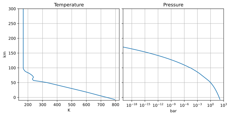
Temperature and pressure

While plotting, we make nice use of the fact that the model uses astropy Quantitys.

fig, axes = plt.subplots(ncols=2, sharey=True, figsize=(8, 4), layout="constrained")
axes[0].plot(model.temperature, model.altitude)
axes[0].set_title("Temperature")
axes[1].plot(model.pressure.to("bar"), model.altitude)  # automatically sets axes units!
axes[1].set_title("Pressure")
axes[1].set_xscale("log")
axes[1].set_xlim(1e-20, 1e3)
axes[1].set_ylim(-10, 300)
for ax in axes:
    ax.grid()

Species molar fraction, polarization, absorption, and refraction

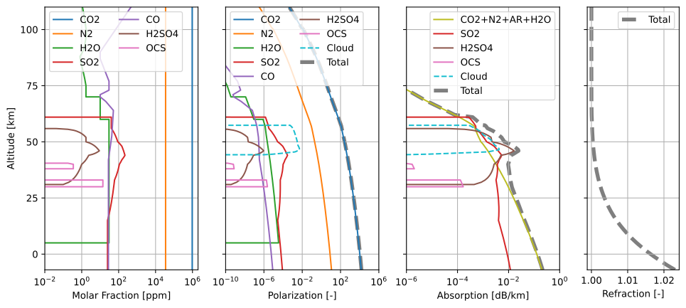
Let’s now plot an overview of the species present in the atmosphere, as well as their contribution to the overall polarization and absorption. Let’s also plot the joint absorption and polarization, and the final refraction profile.

fig, axes = plt.subplots(
    ncols=4, sharey=True, figsize=(12, 5), width_ratios=[5, 5, 5, 3], dpi=300
)
axes[2].semilogx(
    model.absorptions["CO2+N2+AR+H2O"].to("dB/km"),
    model.altitude,
    c=f"C8",
    label="CO2+N2+AR+H2O",
    zorder=2,
)
for i, comp in enumerate(model.molar_fractions.colnames):
    axes[0].semilogx(
        model.molar_fractions[comp], model.altitude, c=f"C{i}", label=comp, zorder=2
    )
    if comp in model.polarizations.colnames:
        axes[1].semilogx(
            model.polarizations[comp] * model.molar_fractions[comp],
            model.altitude,
            c=f"C{i}",
            label=comp,
            zorder=2,
        )
    if comp in model.absorptions.colnames:
        axes[2].semilogx(
            model.absorptions[comp].to("dB/km"),
            model.altitude,
            c=f"C{i}",
            label=comp,
            zorder=2,
        )
axes[1].semilogx(
    model.polarizations["cloud"],
    model.altitude,
    c=f"C9",
    ls="--",
    zorder=2,
    label="Cloud",
)
axes[1].semilogx(
    model.polarization, model.altitude, c=f"C7", lw=4, ls="--", zorder=1, label="Total"
)
axes[2].semilogx(
    model.absorptions["cloud"],
    model.altitude,
    c=f"C9",
    ls="--",
    zorder=2,
    label="Cloud",
)
axes[2].semilogx(
    model.absorption, model.altitude, c=f"C7", lw=4, ls="--", zorder=1, label="Total"
)
axes[3].plot(
    model.refraction, model.altitude, c=f"C7", lw=4, ls="--", zorder=1, label="Total"
)
axes[0].set_xlim(1e-2, 2e6)
axes[0].set_ylim(-7, 110)
axes[1].set_xlim(1e-10, 1e6)
axes[1].set_xlabel("Polarization [-]")
axes[2].set_xlim(1e-6, 1)
axes[2].set_xlabel("Absorption [dB/km]")
axes[0].set_ylabel("Altitude [km]")
axes[0].set_xlabel("Molar Fraction [ppm]")
axes[0].set_yticks(np.arange(0, 101, 25))
axes[3].set_xlabel("Refraction [-]")
for iax, ax in enumerate(axes):
    ax.grid()
    if iax < 2:
        ax.legend(loc="upper left", ncol=2)
    else:
        ax.legend(loc="upper right", ncol=1)

Profile-integrated values

By integrating through the refraction and absorption profiles given a starting (terrain) height, a final (satellite platform) height, and a look angle of the platform (which will correspond to the apparent look angle), we can derive:

• the total signal delay (defined as the difference between the apparent and geometric range),

• the signal attenuation (two-way), which is half of the power absorption,

• the central angle formed by the satellite viewing geometry, and

• the apparent incidence angle at the surface.

Furthermore, from the viewing geometry, we can derive the geometric (in vacuum) range, look angle, and incidence angle. The relevant functions are all vectorized such that we can compute everything in one call.

# range of test values
apparent_look_angle = Quantity(np.linspace(28, 32, num=41), "deg")
height_terrain = Quantity(np.linspace(-6, 16, num=45), "km")
height_platform = Quantity(220, "km")
# combine the two varying quantities in a single grid
grid_terrain, grid_look = np.meshgrid(
    height_terrain.to_value("km"), apparent_look_angle.to_value("rad")
)
# get profile-integrated values
apparent_range, attenuation, central_angle, apparent_incidence_angle = (
    model.get_range_attenuation_angles(
        grid_look.ravel(), grid_terrain.ravel(), height_platform
    )
)
# use law of cosines to get geometric quantities
geometric_range, geometric_look_angle, geometric_incidence_angle = (
    geometry_from_central_angle(central_angle, grid_terrain.ravel(), height_platform)
)
# use it again to get the cross-track displacement
cross_track_displacement = get_cross_track_displacement(
    np.repeat(apparent_look_angle[:, None], height_terrain.size, axis=1).ravel(),
    central_angle,
    grid_terrain.ravel(),
    height_platform,
)
# reshape output into grids again
apparent_range = apparent_range.reshape(grid_terrain.shape)
attenuation = attenuation.reshape(grid_terrain.shape)
central_angle = central_angle.reshape(grid_terrain.shape)
apparent_incidence_angle = apparent_incidence_angle.reshape(grid_terrain.shape)
geometric_range = geometric_range.reshape(grid_terrain.shape)
geometric_look_angle = geometric_look_angle.reshape(grid_terrain.shape)
geometric_incidence_angle = geometric_incidence_angle.reshape(grid_terrain.shape)
cross_track_displacement = cross_track_displacement.reshape(grid_terrain.shape)
# get delay
delay = (apparent_range - geometric_range).to("m")
# get power absorption
power_absorption = 2 * attenuation

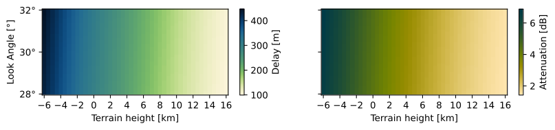
First, we plot the delay and attenuation for the entire range of input terrain and look angles:

fig, axes = plt.subplots(ncols=2, sharey=True, figsize=(10, 1.7))
pc0 = axes[0].pcolormesh(
    height_terrain,
    apparent_look_angle,
    delay.to("m").value,
    cmap=cm.navia_r,
    rasterized=True,
)
pc1 = axes[1].pcolormesh(
    height_terrain,
    apparent_look_angle,
    attenuation.to("dB").value,
    cmap=cm.bamako_r,
    rasterized=True,
)
fig.colorbar(pc0, ax=axes[0], label="Delay [m]")
fig.colorbar(pc1, ax=axes[1], label="Attenuation [dB]")
axes[0].set_ylabel("Look Angle [°]")
# axes[0].set_yticks(np.arange(180, 261, 20))
for ax in axes:
    ax.set_xlabel("Terrain height [km]")
    ax.set_xticks(np.arange(-6, 17, 2))

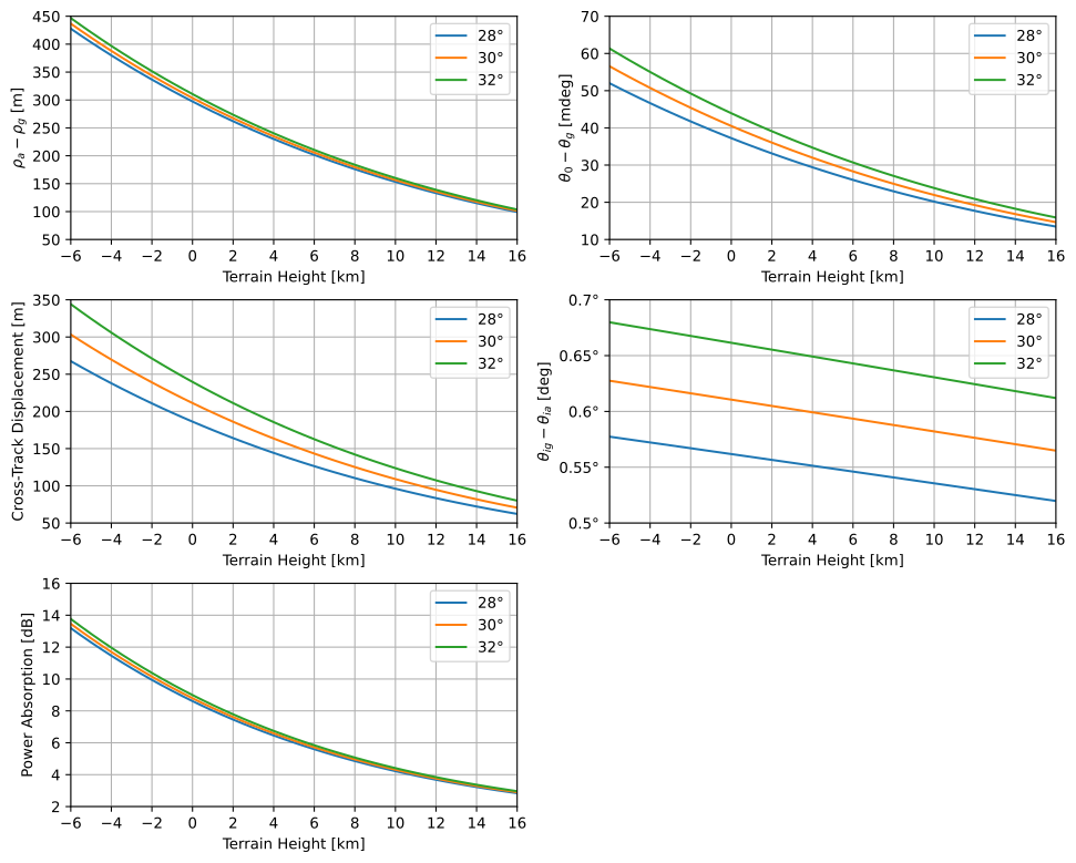
Next, we can extract some terrain-dependent profiles at different look angles:

# create figure
fig, axes = plt.subplots(nrows=3, ncols=2, figsize=(10, 8), layout="constrained")
# loop over look angles
angle_lookup = apparent_look_angle.to_value("°").tolist()
for a in [28, 30, 32]:
    ix = angle_lookup.index(a)
    lbl = f"{a}°"
    # plot delay
    axes[0, 0].plot(height_terrain, delay[ix, :].to("m"), label=lbl)
    axes[0, 0].set_ylim(50, 450)
    axes[0, 0].set_yticks(np.arange(50, 451, 50))
    axes[0, 0].set_ylabel(r"$\rho_a - \rho_g$ [m]")
    # plot look angle difference
    axes[0, 1].plot(
        height_terrain,
        (apparent_look_angle[ix] - geometric_look_angle[ix, :]).to("mdeg"),
        label=lbl,
    )
    axes[0, 1].set_ylim(10, 70)
    axes[0, 1].set_yticks(np.arange(10, 71, 10))
    axes[0, 1].set_ylabel(r"$\theta_0 - \theta_g$ [mdeg]")
    # plot cross-track displacement towards nadir
    axes[1, 0].plot(
        height_terrain,
        cross_track_displacement[ix, :].to("m"),
        label=lbl,
    )
    axes[1, 0].set_ylim(50, 350)
    axes[1, 0].set_yticks(np.arange(50, 351, 50))
    axes[1, 0].set_ylabel("Cross-Track Displacement [m]")
    # plot incidence angle difference
    axes[1, 1].plot(
        height_terrain,
        (geometric_incidence_angle - apparent_incidence_angle)[ix, :].to("°"),
        label=lbl,
    )
    axes[1, 1].set_ylim(0.5, 0.7)
    axes[1, 1].set_yticks(np.arange(0.5, 0.71, 0.05))
    axes[1, 1].set_ylabel(r"$\theta_{ig} - \theta_{ia}$ [deg]")
    # plot attenuation
    axes[2, 0].plot(height_terrain, power_absorption[ix, :].to("dB"), label=lbl)
    axes[2, 0].set_ylim(2, 16)
    axes[2, 0].set_yticks(np.arange(2, 17, 2))
    axes[2, 0].set_ylabel("Power Absorption [dB]")
# last axis off
axes[2, 1].set_axis_off()
# make pretty
for ax in axes.ravel()[:-1]:
    ax.set_xlim(-6, 16)
    ax.set_xticks(np.arange(-6, 17, 2))
    ax.set_xlabel("Terrain Height [km]")
    ax.grid()
    ax.legend()

Example of non-default model parameters

Let’s also have a look at a non-default parameter settings, and how it can affect the final delay and attenuation values. We do this for the example of the H2SO4 mixing ratio in the atmosphere, for which there are both original and reprocessed datasets available. These are accessible through the parameter profile_H2SO4 of the Duan2010 class.

We do this by creating a new model object with a non-default setting, computing the path-integrated delay and attenuation values again, and then subtracting them from the values we got from the default model:

# load a different H2SO4 profile
from xvamp.references.magellan321x import h2so4_mr_x_3214

# new model object
model_new = Duan2010(profile_H2SO4=h2so4_mr_x_3214)
# get profile-integrated values
delay_new, attenuation_new = model_new.get_delay_attenuation(
    grid_terrain.ravel(), height_platform, grid_look.ravel()
)
delay_new = delay_new.reshape(grid_terrain.shape)
attenuation_new = attenuation_new.reshape(grid_terrain.shape)

fig, axes = plt.subplots(ncols=2, sharey=True, figsize=(10, 1.7))
pc0 = axes[0].pcolormesh(
    height_terrain,
    apparent_look_angle,
    (delay_new - delay).to("mm").value,
    cmap=cm.batlow,
    rasterized=True,
)
pc1 = axes[1].pcolormesh(
    height_terrain,
    apparent_look_angle,
    (attenuation_new - attenuation).to("dB").value,
    cmap=cm.lipari,
    rasterized=True,
)
fig.colorbar(pc0, ax=axes[0], label="ΔDelay [mm]")
fig.colorbar(pc1, ax=axes[1], label="ΔAttenuation [dB]")
axes[0].set_ylabel("Look Angle [°]")
for ax in axes:
    ax.set_xlabel("Terrain height [km]")
    ax.set_xticks(np.arange(-6, 17, 2))

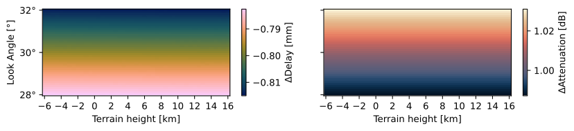
Here, we can see that there is a significant difference in the expected attenuation of the radar signal: over 1 dB! Going back to the datasets we tested, we compared an older source for the H2SO4 mixing ratio [Jenkins, 1996] (processing details in [Jenkins et al., 1994]) with the default one from Duan et al. [2010], which is based on the reprocessed data of Jenkins et al. [2002]. The different attenuation is, as expected, due to the large difference in H2SO4 mixing ratio:

# create figure
fig, ax = plt.subplots()
# add H2SO4 mixing ratios for both models
ax.plot(model.molar_fractions["H2SO4"], model.altitude, label="Default (reprocessed)")
ax.plot(
    model_new.molar_fractions["H2SO4"], model_new.altitude, label="Orbit 3214 (old)"
)
# make pretty
ax.set_xlabel("H2SO4 Mixing Ratio [ppm]")
ax.set_ylabel("Altitude [km]")
ax.set_ylim(30, 60)
ax.legend()

<matplotlib.legend.Legend at 0x7f717de06900>

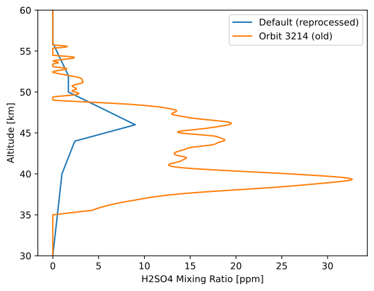
While the default dataset contains less H2SO4, therefore less attenuation, and therefore a more favorable case for the VISAR instrument operations, it is chosen as the default since it is a newer, reprocessed dataset, and we can therefore expect it to be more accurate. The other profiles are included as options in case we want to challenge the different input assumptions. Other options are available and documented in xvamp.model.Duan2010.