Model Verification#
This notebook collects some experiments used to verify the validity of the default xvamp.models.Duan2010 model.
Note: There are a couple of options that can modify the default xvamp.models.Duan2010 behavior, which are documented in the API, but not shown here.
Venus Brightness Temperature#
There exist measurements of the brightness temperature of Venus in the literature
[Ho et al., 1966], and our atmospheric model includes (almost) everything we need
to compute one ourselves. So, the brightness temperature is a natural approach to
verify that our model is physically consistent. The brightness temperature can be
computed with get_brightness_temperature(), which is based on
Ulaby and Long [2013].
We start by initializing our default model:
[1]:
# some basic imports
import numpy as np
import matplotlib.pyplot as plt
from cmcrameri import cm
from astropy.units import Quantity, dimensionless_unscaled
from astropy.visualization import quantity_support

# import reference model
from xvamp.models import Duan2010

# instantiate
model = Duan2010()

# initialize pretty plotting
quantity_support()
%config InlineBackend.figure_formats = ["svg", "pdf"]
The brightness temperature calculation requires the knowledge of the brightness temperature at the surface, which is not something our model can compute. However, we know the temperature of the atmosphere at the surface, and the surface should be somewhat equilibrated with that temperature. So, we simply test our model using a range of surface brightness temperatures that are derived from the atmosphere’s temperature through the surface emissivity:
[2]:
# import brightness computation function
from xvamp.geometry import get_brightness_temperature

# define range of emissivities to apply to atmosphere temperature
# to derive surface brightness temperature
emissivity = np.linspace(0.5, 1.0, num=51)

# select some altitude levels for which to compute everything
ix_alt = np.arange(1, 15, 2)

# define range of surface brightness temperatures to assume
T_B_surface = emissivity[:, None] * model.temperature[ix_alt][None, :]

# for each assumed element in T_B_surface, get the total brightness temperature
T_B = Quantity(
    [
        get_brightness_temperature(
            model.altitude[i:],
            model.temperature[i:],
            model.refraction[i:],
            model.absorption[i:],
            Quantity(30, "°"),
            T_B_surface[:, ii],
        )
        for ii, i in enumerate(ix_alt)
    ]
)
In the following figure, we show the computed brightness temperatures of the entire planet given the different surface brightness temperatures i.e., surface emissivities) we assume. We also add the range of possible brightness temperatures derived by Ho et al. [1966], Fig. 13, around the VISAR frequency of 7.9 GHz.
[3]:
# import plotting functionality
from matplotlib.colors import Normalize

# start with the Ho & Kaufman ranges for X-band
plt.axhspan(Quantity(578, "K"), Quantity(657, "K"), fc="k", alpha=0.1, ec=None)
plt.axhspan(Quantity(500, "K"), Quantity(660, "K"), fc="k", alpha=0.1, ec=None)
# add our derived curves, colored by terrain altitude
norm = Normalize(
    vmin=model.altitude[ix_alt[0]].value, vmax=model.altitude[ix_alt[-1]].value
)
for ii, i in enumerate(ix_alt):
    plt.plot(
        emissivity,
        T_B[ii, :],
        c=cm.batlow(norm(model.altitude[i].value)),
        lw=2,
        label=f"{model.altitude[i]:.0f}",
    )
# make pretty
plt.xlabel("Surface Emissivity [-]")
plt.ylabel("Brightness Temperature [K]")
plt.legend(ncol=2)
plt.xlim(emissivity[0], emissivity[-1])
plt.ylim(400, 800)
[3]:
(400.0, 800.0)
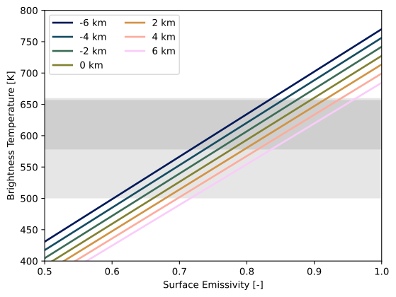
This figure shows, for each terrain altitude, the range of planetary brightness temperatures we get by varying the assumed surface brightness temperature (defined through the surface emissivity). The good thing is that there is a wide range of emissivities (approx. 0.72 to 0.82) where all curves lie within the wider shaded area. That shaded area is one range of possible brightness temperatures as shown by Ho et al. [1966], Fig. 13. The narrower shaded area is a different possible range, and while there is no single factor where all curves lie within it, our curves are still plausible as it is certainly possible to have different average surface brightness temperature factors at different altitudes and geographic locations.
Indeed, Pettengill et al. [1992] report radar-wavelength emissivities (those we are sensitive to) that for a wide fraction of the Venus surface are between approx. 0.8 and 0.9. In some specific areas, they can be as low as 0.5. In general, however, this comparison shows that out atmospheric model is consistent with what the literature reports as brigthness temperatures and surface emissivities.
Model Intercomparison#
There are few other datasets available for us to compare the final refraction and absorption profiles provided by XVAMP to. One is Stratton [1968], who derived refraction profiles from in-situ measurements complemented by laboratory-derived parameters. The other is the radio occultation experiment aboard the Magellan mission, processed by Jenkins et al. [1994], which contains both refraction [Jenkins, 1996] and absorption [Jenkins, 1996].
For this section, we will follow the verification settings in the reference code,
which are designed to offer as close to a comparison with the Magellan data as
possible. To distinguish between the default model and the non-default model derived
for this verification section, we name them “Defaults” and “Verification”, respectively.
For “Verification”, we diverge from the default temperature, H2O, CO, SO2, H2SO4, and
OCS profiles, and select simpler ones. In particular, the H2SO4 profile is not the
one derived for global use, but one derived from the Magellan data itself.
We also neglect the influence of the clouds. There is a shorthand to the “Verification”
case of the model, available in
Duan2010Verification.
[4]:
# import the Magellan radio occultation results as well as the Stratton (1968)
# analytic refraction model
from xvamp.references import magellan321x, stratton_1968
Refraction#
The Stratton (1968) analytic model is then evaluated on “Verification“‘s profiles, namely the temperature profile as well as the partial pressures of CO2 and H2O. The Magellan experiment results are simply loaded. Finally, both the Stratton and Magellan values are converted to the real part of the relative permittivity for comparison with the XVAMP model.
[5]:
# import verification-settings model
from xvamp.models.duan_et_al_2010 import Duan2010Verification

# initialize non-default XVAMP model
model_verification = Duan2010Verification()
# this is equivalent to using
# from xvamp.references import duan_et_al_2010 as duan2010figures
# from xvamp.references import kolodner_steffes_1998
# model_verification = Duan2010(
#     profile_TPD="seiff:75",
#     profile_H2O=duan2010figures.h2o_old_molar_fraction,
#     profile_SO2=duan2010figures.so2_old_molar_fraction,
#     profile_CO=duan2010figures.co_old_molar_fraction,
#     profile_H2SO4=kolodner_steffes_1998.h2so4_mr_3212,
#     profile_OCS=duan2010figures.ocs_old_molar_fraction,
#     use_clouds_from="none",
# )

# load Magellan data
mgn_abs, mgn_rtpd = magellan321x.get_wavelength_orbit("X", 3212)
# convert mean and plus/minus 3 s.d.
mgn_epsprimer = mgn_rtpd["REFRACTIVITY"].to(dimensionless_unscaled) ** 2
mgn_epsprimer_lower = (mgn_rtpd["REFRACTIVITY"] - 3 * mgn_rtpd["REFRACT_DEV"]).to(
    dimensionless_unscaled
).value ** 2
mgn_epsprimer_upper = (mgn_rtpd["REFRACTIVITY"] + 3 * mgn_rtpd["REFRACT_DEV"]).to(
    dimensionless_unscaled
).value ** 2
# evaluate Stratton model
stratton_epsprimer = (
    stratton_1968.get_refractivity(
        model_verification.temperature,
        model_verification.pressure * model_verification.molar_fractions["CO2"],
        model_verification.pressure * model_verification.molar_fractions["N2"],
        model_verification.pressure * model_verification.molar_fractions["H2O"],
    ).to(dimensionless_unscaled)
    ** 2
)
[6]:
plt.plot(
    model.relative_permittivity.real,
    model.altitude,
    label="Defaults",
)
plt.plot(
    model_verification.relative_permittivity.real,
    model_verification.altitude,
    label="Verification",
)
plt.plot(
    mgn_epsprimer,
    mgn_rtpd["ALTITUDE"],
    ls="--",
    label="Magellan orbit 3212 ± 3σ",
)
plt.fill_betweenx(
    mgn_rtpd["ALTITUDE"].to("km").value,
    mgn_epsprimer_lower,
    mgn_epsprimer_upper,
    fc="C1",
    alpha=0.2,
)
plt.plot(
    stratton_epsprimer,
    model_verification.altitude,
    ls=":",
    label="Stratton (1968)",
)
plt.xlabel("Real Part of the Relative Permittivity [-]")
plt.xlim(1, 1.004)
plt.ylabel("Altitude [km]")
plt.ylim(34, 98)
plt.legend()
[6]:
<matplotlib.legend.Legend at 0x7fe615f2f620>
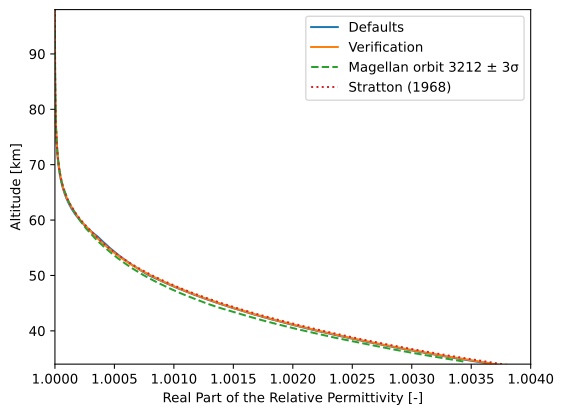
As we can see, the XVAMP profiles closely match both the Stratton model and the Magellan dataset. At this scale, for the real part of the relative permittivity, the model settings “Defaults” and “Verification” do not yield meaningful differences.
Absorptivity#
Next up is the absorptivity. We start from the same two “Defaults” and “Verification” model settings.
There are three other non-default models we would like to add, however - again to showcase the influence of the assumed H2SO4 profile. In the “Verification” case from above, we used the H2SO4 profile of orbit no. 3212 but reprocessed as published in Kolodner and Steffes [1998] (KS98 in the plots below). By contrast, the “Defaults” case uses a profile from Jenkins et al. [2002] but further adapted by Duan et al. [2010] (D10 below).
Two models we want to add are both derived from the “Verification” case. The first one uses the Duan et al. [2010] (D10) H2SO4 profile. The second one uses the H2SO4 profile from the original radio occulatation experiment as published in Jenkins [1996] (J96 below). The difference between J96 and KS98 is only that KS98 reprocessed the original data, and found a different result. Finally, we add a model based on the “Defaults” case, but use KS98 as the H2SO4 profile.
[7]:
# import other profiles to test
from xvamp.references import (
    duan_et_al_2010 as duan2010figures,
    kolodner_steffes_1998,
    magellan321x,
)

# get multiple profiles for comparison of the H2SO4 impact
m_ks98 = Duan2010(profile_H2SO4=kolodner_steffes_1998.h2so4_mr_3212)
m_ver_d10 = Duan2010Verification(profile_H2SO4=duan2010figures.h2so4_molar_fraction)
m_ver_j96 = Duan2010Verification(profile_H2SO4=magellan321x.h2so4_mr_x_3212)
We now have all the different validation test cases, and plot their absorptivity profiles. We also add a plot of the part of the absorptivity that comes from the H2SO4 constituent, as it is one of the biggest drivers and will allow us to investigate the results better.
[8]:
plt.figure(figsize=(7, 5), layout="constrained")
plt.plot(
    mgn_abs["ABSORPTIVITY"],
    mgn_abs["ALTITUDE"],
    c="k",
    label="Measured Magellan orbit 3212 ± 3σ",
)
plt.fill_betweenx(
    mgn_abs["ALTITUDE"].to("km").value,
    (mgn_abs["ABSORPTIVITY"] - 3 * mgn_abs["ABSORP_DEV"]).to_value("dB/km"),
    (mgn_abs["ABSORPTIVITY"] + 3 * mgn_abs["ABSORP_DEV"]).to_value("dB/km"),
    fc="k",
    alpha=0.2,
)
batlow_res = cm.batlow.resampled(8)
for i, (mdl, mdl_name, c) in enumerate(
    zip(
        [model, m_ks98, m_ver_d10, model_verification, m_ver_j96],
        [
            "Defaults (H2SO4 from D10)",
            "Defaults (except H2SO4 from KS98)",
            "Verification (except H2SO4 from D10)",
            "Verification (H2SO4 from KS98)",
            "Verification (except H2SO4 from J96)",
        ],
        [batlow_res(1), batlow_res(2), batlow_res(4), batlow_res(5), batlow_res(6)],
    )
):
    plt.plot(
        mdl.absorption.to_value("dB/km"),
        mdl.altitude,
        c=c,
        label=mdl_name,
    )
    plt.plot(
        mdl.absorptions["H2SO4"].to_value("dB/km"),
        mdl.altitude,
        c=c,
        ls="--",
    )
plt.grid()
plt.xlabel("Absorptivity [dB/km]")
plt.xlim(-0.02, 0.08)
plt.ylabel("Altitude [km]")
plt.ylim(35, 60)
plt.legend()
plt.title(
    "Total (solid) and H2SO4 contribution (dashed) for different\n"
    "test cases compared with orbit 3212 Magellan measurements"
)
[8]:
Text(0.5, 1.0, 'Total (solid) and H2SO4 contribution (dashed) for different\ntest cases compared with orbit 3212 Magellan measurements')
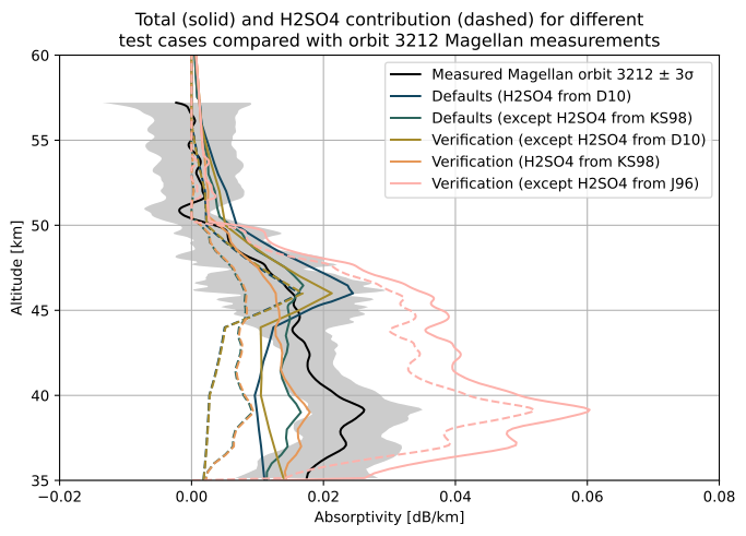
This plot is busy, so let’s break it down. In black is the measured Magellan orbit 3212 absorptivity profile including the reported uncertainty (plotted is three times the standard deviation). Ideally, our XVAMP model(s) will fall into the grey area.
The two validation test cases that use the D10 H2SO4 profiles decently fit the data above 45 km altitude, but underestimate the absorptivity below 45 km. For the two cases that use H2SO4 profiles derived from the experiment data itself (J96 and KS98), we find that KS98 indeed does a good job, and only scratches the three-standard-deviations boundary below 45 km altitude. (KS98 is also the profile used for the verification plot Fig. 10 in the Duan et al. [2010].) The orbit 3212 profile from J96 contains much more H2SO4, and yields a vastly higher absorptivity profile.
To summarize, we would therefore argue that our model, for the test case that most closely resembles the conditions measured / expected for Magellan’s orbit 3212 (namely the KS98 profile), reproduces to a satisfying degree the absorptivity profile reported by the radio occultation experiment.
To assess, however, the overall impact on the mission design if one were to assume one of the non-default profiles, let’s have a closer look at the following models:
The blue “Defaults (H2SO4 from D10)”, i.e., all default settings in the model
The green “Defaults (except H2SO4 from KS98)”, where we only swap the assumed H2SO4 profile
The orange “Verification (H2SO4 from KS98)”, which mimics the verification settings of Duan et al. [2010]
We then compute all profile-integrated values of the range delay and attenuation, and subtract the reference model to show the differences.
[9]:
# range of test values
apparent_look_angle = Quantity(np.linspace(28, 32, num=41), "deg")
height_terrain = Quantity(np.linspace(-6, 16, num=45), "km")
height_platform = Quantity(220, "km")
# combine the two varying quantities in a single grid
grid_terrain, grid_look = np.meshgrid(
    height_terrain.to_value("km"), apparent_look_angle.to_value("rad")
)
# get profile-integrated values
ref_delay, ref_attenuation = (
    out.reshape(grid_terrain.shape)
    for out in model.get_delay_attenuation(
        grid_terrain.ravel(), height_platform, grid_look.ravel()
    )
)
# initialize plot
fig, axes = plt.subplots(ncols=2, nrows=2, figsize=(10, 3.4), layout="constrained")
# loop over other models
for i, (mdl, mdl_name) in enumerate(
    zip(
        [m_ks98, model_verification],
        ["Defaults (except H2SO4 from KS98)", "Verification (H2SO4 from KS98)"],
    )
):
    # compute
    mdl_delay, mdl_attenuation = (
        out.reshape(grid_terrain.shape)
        for out in mdl.get_delay_attenuation(
            grid_terrain.ravel(), height_platform, grid_look.ravel()
        )
    )
    # get difference
    diff_delay_m = (mdl_delay - ref_delay).to("mm").value
    diff_attenuation_dB = (mdl_attenuation - ref_attenuation).to("dB").value * 1000
    # plot
    pc0 = axes[i, 0].pcolormesh(
        height_terrain,
        apparent_look_angle,
        diff_delay_m,
        cmap=cm.batlow,
        rasterized=True,
    )
    pc1 = axes[i, 1].pcolormesh(
        height_terrain,
        apparent_look_angle,
        diff_attenuation_dB,
        cmap=cm.lipari,
        rasterized=True,
    )
    axes[i, 0].set_title(mdl_name)
    axes[i, 1].set_title(mdl_name)
    fig.colorbar(pc0, ax=axes[i, 0], label="ΔDelay [mm]")
    fig.colorbar(pc1, ax=axes[i, 1], label="ΔAttenuation [mdB]")
for ax in axes.flat:
    ax.set_ylabel("Look Angle [°]")
    ax.set_xlabel("Terrain height [km]")
    ax.set_xticks(np.arange(-6, 17, 2))
fig.suptitle("Comparison of All-Defaults Model with...")
[9]:
Text(0.5, 0.98, 'Comparison of All-Defaults Model with...')
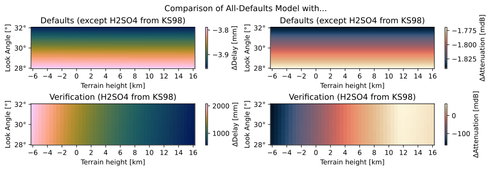
The takeaway here is that simply using the H2SO4 profile from the Magellan orbit as derived by KS98 does not have a big impact on the integrated values. The verification model can have upto 1.5 m additional range delay, but upon further inspection, this is more likely due to constituent profile differences at lower altitudes, where this model may not be applicable. Still, it is good to know what the impact of other profiles could be.